Turbidity sensor calibration and Formazin problems

In the previous post, I was walking through some past bad designs and how they ultimately lead to our latest prototype (prototype 2.0). In this post, I would like to explain the turbidity sensor calibration method. First, how to calibrate to NTU using Formazin and which regression model to choose. Then I would like to explain the calibration from NTU to SSC. I will then highlight some problems we found with Formazin calibration. Finally, I will suggest a better calibration for these sensors.

Formazin turbidity sensor calibration steps

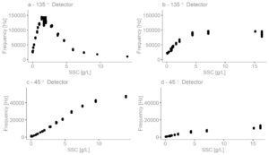
To begin the turbidity sensor calibration, we made several dilutions of Formazin, a popular calibration liquid for turbidity sensors. The Formazin that we purchased is rated at 4000NTU and we created dilutions using deionized water: 0, 3, 6, 10, 40, 70, 100, 400, 700, 1000, 2000, and 4000 NTU, as is commonly done in turbidity sensors. I then poured each dilution into prototype 1.0 and took measurements. The detectors in the sensor recorded the measurements in Hz (Hz frequency is proportional to the observed light intensity). You can find more details about the sensor design and its operating principle in this post.

Model selection based on prototype 1.0

In the previous post, we conducted three different experiments with Formazin. Using those results, I made various multiple linear regression models for NTU ~ observed light intensity. The four models applied to prototype 1.0 are of the type:

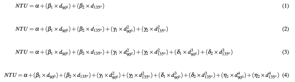
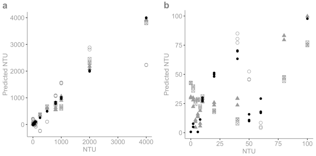
where d_135° and d_45° is the quantity of light detected by detectors at angles 135° and 45° respectively, alpha is the y-intercept, and β_1,2 – η_1,2 are the regression coefficients. The figure to the right shows the results of all four of these models.

We see in this figure to the right that for the full range of data, none of the given models are able to accurately predict NTU except for the fourth-order. The fourth-order model is able to predict down to 250 NTU but its unable to predict below 250 NTU. Most likely, to calibrate this sensor in the full 0-4000 NTU range we should create a separate model for the 0-250 NTU range. The final calibration for this sensor would be two models. One in the 0-250NTU range and a fourth-order model in the 250-4000NTU range.

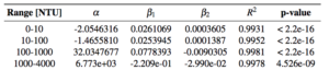
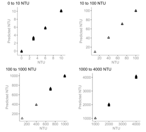
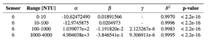
There are probably a thousand different variations of working models that we can make. And due to the unnecessary complexity of the fourth-order model, we instead fitted the data using the simplest multiple linear regression model in four different ranges (0-10NTU, 10-100NTU, 100-1000NTU, 1000-4000NTU). Since this is often done by commercial turbidity sensors. The model is of the form:

where α is the y-intercept, and β_1 and β_2 are the coefficients associated with the first detector (d_45°) and second detector (d_135° ), respectively. The model coefficients are in the table below.

Calibration of prototype 2.0

I tried to calibrate our second prototype (the waterproof one used in our mixing tank experiments) the same way as I calibrated prototype 1.0. I tried this by creating a multiple regression model in four ranges (0-10NTU, 10-100NTU, 100-1000NTU, 1000-4000NTU) using the response from both detectors (d_45° and d_135°). And just as in prototype 1.0, this appears to work. Until you want to use the sensors in “real” sediment. I will explain further…

When we calibrate with Formazin, we obtain a multiple regression model by using the responses of both detectors (NTU = f(d45,d135). I have tried my best to provide a visual representation in the image to the left.

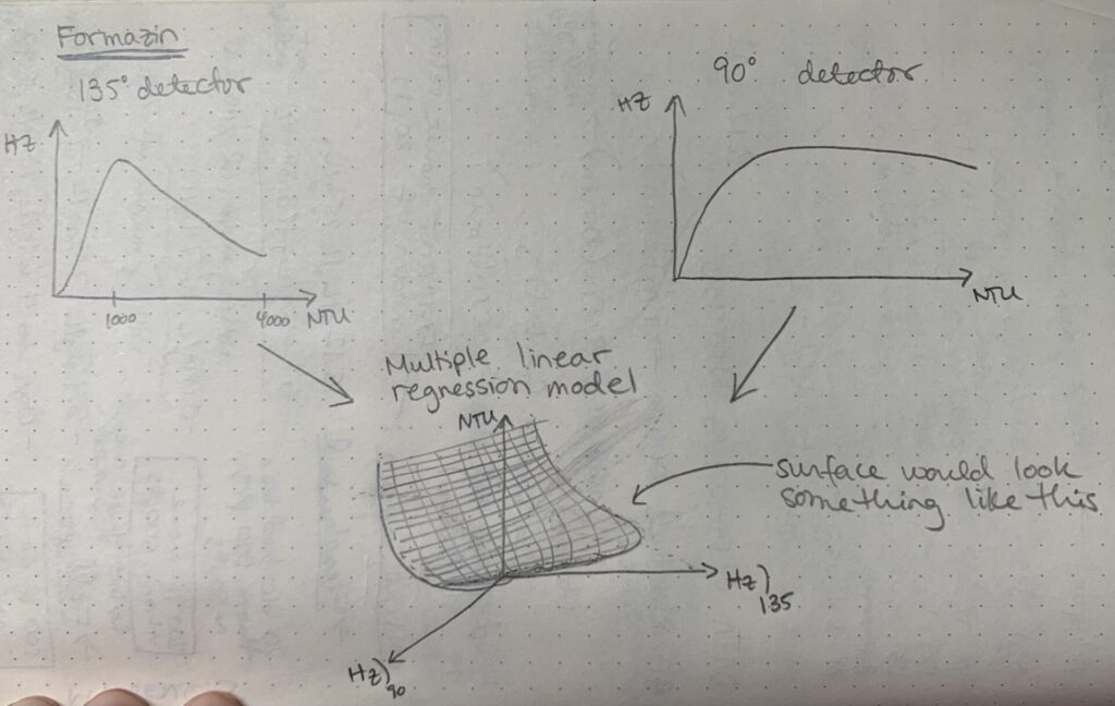
As we subsequently use this sensor+model to measure water+sediment, we hope that each detector will behave in sediment as it behaves in Formazin (and output the same NTU~Hz curve). However, this is not the case because Formazin scatters light evenly in all directions. And this is not true in natural sediment where the directionality of scattered light is highly sensitive to particle grain size and shape.

Directionality of scattered light

To understand this concept better, look at the key figure to the right. Here I have plotted the light intensity response from both detectors (d_45° and d_135°) for two different sediments types. a) Feldspar milled for pottery that has a d50=30um and a rho=2.65g/cm3. And b) Fieschertal sediments from the deposits in the tailwater channels at the Fieschetal hydropower plant (HPP) in the Canton of Valais, Switzerland. This sediment has a d50=90um and rho=2.7g/cm3.

The 135° detector sees a light peak in Feldspar powder, whereas there is no peak in Fieschertal powder. The 45° detector shows a linear increase in the amount of light received in both sediments. But the quantity of light received by the detector in Feldspar is much higher than in Fieschertal sediment. Matos et al. (2019) found similar results previously.

According to Sadar (1998) and Tran et al. (2006), particles with sizes much smaller than the wavelength of the incident light will scatter light with roughly equal intensity in all directions. Particles larger than the wavelength of the incident light will create a spectral pattern that results in greater light scattering in the forward direction than in the other directions. Therefore, the reported differences in NTUs in Feldspar and Fieschertal sediment (key figure) are likely due to the shape and size of the two sediment types. And their detector responses are different than Formazin because Formazin is a polymer that scatters light evenly in all directions.

Due to this directionality of scattered light, the detectors output a different NTU~Hz curve for every sediment type. So at 1000 NTU in Formazin, d_135° and d_45° can output 10000Hz and 5000Hz, respectively and land somewhere on the calibration surface object. However, let’s say that we have a sediment+water mixture and the detectors read d_135°=2500Hz and d_45°=5000Hz, where does this fall on our calibration surface? At which NTU is this sediment+water mixture?

With every test that I did in water+sediment, I got ridiculously large (positive and negative) NTU values because the d_135° and d_45° readings never landed on the calibration surface. For this reason, moving forward with this model was impossible.

Model chosen for prototype 2.0

We know from the discussion above that using a model with two detectors to measure both Formazin and different sediments doesn’t work well. So in order to have a model which works in both Formazin and natural sediments, I rebuilt the calibration model but only using the 45° detector. The model is of the form:

where α is the y-intercept, β is the first order coefficient associated with the measured light intensity from the 45° detector and γ is the second-order coefficient from the same detector. In the figure below, we can see the resulting models along with their coefficients:

Again, this is not the only model we can use for this type of calibration. Here, I simply chose a linear regression in four distinct ranges because that’s what I did for prototype 1.0. However, although we have found a model that “works” (e.g. gives us reasonable results) it doesn’t mean that the results are right. We know this from our key figure, where the 45° detector response curve changes with different sediment types. Meaning that even with our new working model made from Formazin, the measured NTU will probably have significant errors in natural sediments.

I try to address this problem in the last section of this blog post.

Turbidity sensor calibration of NTU to SSC

NTU as a unit of measure of turbidity is not intuitive for monitoring SSC since it is not universally comparable between watersheds. For example, you cannot assume that 1000 NTU in two different rivers means they have the same SSC [g/L]. This is because turbidity does not only depend on SSC, but also on the Particle Size Distribution (PSD), shape, and particle material properties such as colour (reflectivity), density, refractive index, and surface roughness (Downing, 2006; Gippel, 1995; Sutherland, 2000).

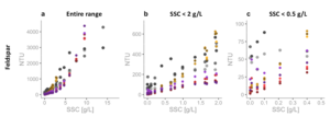
We built 8x prototype 2.0’s and tested them in a mixing tank with various sediment types and SSCs. The figure above shows the performance of our prototype 2.0 in Feldspar (taken from our preprint). We see that the relationship between NTU and SSC is linear in the sub 2 g/L range and becomes non-linear with increasing SSC. Holliday et al. (2003) and several others (Baker et al., 2001; Matos et al., 2019) had observed something similar. Kelley et al. (2014) tried to use a linear model to calibrate NTU and SSC but had to split their model into several ranges of NTU. Holliday et al. (2003) found through experiments that the relationship between turbidity and SSC follows:

where a and b are regression-estimated coefficients and b is approximately equal to one for all particles. But in general, for every watershed and sediment type, it is likely that both a and b will be different. For example, Costa et al. (2018) found a = 0.56 and b = 1.25 in their investigated alpine catchment. Whereas Felix et al. (2018) found a = 0.59 and b = 1 in their HPP storage tunnel. In our case, at larger SSCs the relationship diverges from linearity. Therefore, when working with these sensors it’s important to realize that a doubling in SSC can mean a doubling in NTU at lower NTUs and a quadrupling at higher NTUs. For example, 1 to 2 g/L can give 100 to 200 NTU but 10 to 20 g/L can give 1000 to 4000 NTU.

Additional problems with Formazin

Many processes are hidden in the NTU unit

A sensor that simply provides a clarity estimate can undergo a calibration to NTU with formazin. This is the traditional turbidity sensor calibration. And our open-sourced sensors can also be used and calibrated in this way. However, within this unit of measure is hidden many complex processes, such as particle size, configuration, refractive index, organic matter and other floating debris, algae, air bubbles and water discoloration (wavelength absorption), which all determine the spatial distribution of the scattered light intensity around a particle (Sadar, 1998; Dabney et al., 2006). It is very difficult to decipher these processes from an NTU unit.

Kitchener et al. (2017) has shown that NTU is not a physically valid unit of turbidity and suggests recording data in the SI unit of radiated intensity [mW/sr] (Kitchener et al., 2019). Since the traditional calibration is based on the mass-concentrations of arbitrary polymer suspensions (e.g. Formazin), and not on the intrinsic optical properties of the particles in suspension. This is also what we see in the key figure mentioned previously. Traditional calibration cannot determine what elements cause the water’s clarity to change. Instead, a solution may be to calibrate one of our sensors directly to SSC. And additionally, equip it with other detectors to determine, for example, the presence of organic matter. This is what Matos et al. (2019) achieved when they equipped a 90° light scatter detector with a UV transmitter and receiver.

Temporal variation in PSD affects the sensors

Another issue noted by Felix et al. (2015) is that during a flood event, commercial NTU-calibrated turbidimeters yielded up to 80% lower SSCs than those from Laser in-situ Scattering and Transmissometry (LISST) and bottle samples when coarser particles were present. They mainly attribute this to the temporal variation in PSD; as coarser particles produce less attenuation and scattering at a given SSC (as we see with Fieschertal sediment in the key figure). For this reason, they recommend more advanced optical techniques for SSC such as LISST or Coriolis Flow- and Density Meter (CFDM). They found that these devices were less biased by temporary PSD variations than SSCs obtained by turbidimeters. However, these devices are generally unsuitable for field applications. They also raise the measurement costs to US$ 15 000 – 25 000 (for a CFDM (Felix et al., 2016; Rai and Kumar, 2015)) and between US$ 35 000 and 100 000 (for LISST (Rai and Kumar, 2015)).

In their experiments, Felix et al. (2018) used a turbidimeter that was calibrated up to 4000NTU. They found that their NTU-SSC calibration was only valid for particles up to d_50 = 17μm. The variation in PSD isn’t an issue when the particles present are relatively fine (Felix et al., 2016) (our feldspar and fieschertal sediment have d_50=30um and d_50=90um, respectively). They found that the coarsest particles followed a hysteresis pattern in transport, affecting the NTU-SSC calibration when particles were coarser than d50 = 17μm. They also saw no clear correlation between SSC and d_50. However, they did find that the slope of their NTU-SSC calibration curve (eqn. 6 (Felix et al., 2018)) decreases with coarser particles (as seen in our Fig.2 in our preprint).

Therefore, PSD will affect our turbidity sensor calibration and measurements since our sensors do not measure PSD. But by directly calibrating Hz-SSC, we can obtain a regression fit that spans the entire particle size range; more accurately representing the “true” SSC and overcoming the limitation imposed by the manufacturer’s standard Hz-NTU calibration. Additionally, we may further improve the Hz-SSC relation with multiple samples obtained during various flood events when larger particles are transported. And measuring at a suitably high frequency and time-averaging can reduce random errors due to temporal fluctuations in PSD (Felix et al., 2018). It would be worth investigating whether our site-specific Hz-SSC calibration can consistently capture SSC as both LISST and CFDM (Felix et al., 2016). We conceptually demonstrate this new calibration method in the next section.

Better turbidity sensor calibration

We challenge the need to calibrate the sensors to NTU and using a separate NTU-SSC relation to predict SSC. Since our sensors are meant for a range of different rivers with various grain sizes and shapes. Therefore, the environment (the direction of scattered light and PSD) is constantly changing. We envision that one can directly calibrate SSC observations to the reflected light intensity (Hz) observed by the combined detectors (d_135° and d_45°). We do this by measuring suspended sediment concentration in a few samples that cover a range of SSCs. You can do this in either a laboratory calibration experiment or in on-site river applications.

In this approach, we calibrated the light intensity measured by the detectors for each open-source sensor directly to SSC. We did this separately for the Feldspar and Fieschertal sediment. The model used is of the form:

where α is the y-intercept, d_1 is the light intensity measured by the 45° detector, d_2 is the light intensity measured by the 135° detector β1,2-η1,2 are the 1st-4th order coefficients associated with d1 and d2. Figure 6 in our preprint shows SSC mean predictions against observations for all eight versions of the sensor. The fit is excellent across the entire range of SSC with R2 >0.98, with the main benefit due to the multiple linear regression using both detectors. Analyzing the versions separately, all sensors are now able to predict well in the entire SSC range. We could probably make an improvement in the 0-0.5g/L range by splitting the model and having two separate linear calibrations.

It is important to note that avoiding the Formazin calibration step has additional benefits. By calibrating the detector output directly to SSC, we are able to save up to a week’s worth of lab work. Additionally, we are able to avoid exposure to Formazin, a known carcinogen. Collecting gravimetric samples and calibrating directly to SSC might seem like a lot of work. But anyone would need to do this anyways when installing turbidity sensors in a river network to collect SSC data.

Conceptual example of a better calibration

We conceptually demonstrate the direct turbidity sensor calibration to SSC in a real case below. This calibration gives a more representative SSC reading and is shown in the conceptual image. From Monday to Saturday, isolated rainfall events occur only in certain subcatchments, as the image depicts. Each subcatchment has a different grain size distribution and different grain properties. This causes light to scatter differently (creating different scatter spectra). A sensor is located near the outlet of a catchment. The sensor works by measuring the quantity of scattered light (at an angle) and it is consistently measuring this value. A rainfall event on Monday in a subcatchment with very fine particles gives rise to an SSC of 10g/L at the sensor location. The SSC is determined gravimetrically from a bottle sample. However, these fine particles do not scatter light strongly in the direction of the sensor detector. This causes the calibration points to sit above our calibration curve (low light detected – similar to Feldpsar). Whereas, a rainfall event on Saturday in a subcatchment with very coarse particles, giving rise to an SSC of 15g/L. This SSC scatters light strongly in the direction of the sensor detector (even more than is expected at this SSC). This causes the calibration points to sit below our calibration curve (higher amount of light detected – similar to Fieschertal).

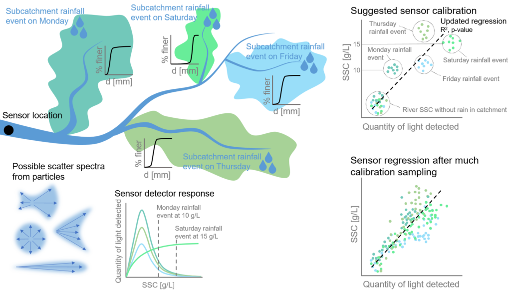
The combination of response curves from multiple detectors can produce good reflectance curves for a range of sediment types (sources) and concentrations. The mixing of these response curves over many events should lead to a robust calibration curve for the entire catchment. And also include individual subcatchments and reaches where one can make distributed measurements. In this way, we can identify sediment sources with possibly different sediment properties.

References

Matos, T., Faria, C. L., Martins, M. S., Henriques, R., Gomes, P. A., & Goncalves, L. M. (2019). Development of a cost-effective optical sensor for continuous monitoring of turbidity and suspended particulate matter in marine environment. Sensors, 19(20), 4439.

Sadar, M. J. (1998). Turbidity science. Technical Information Series—Booklet no. 11. Hach Co. Loveland CO, 7, 8.

Tran, N. T., Campbell, C. G., & Shi, F. G. (2006). Study of particle size effects on an optical fiber sensor response examined with Monte Carlo simulation. Applied optics, 45(29), 7557-7566.

Downing, J. (2006). Twenty-five years with OBS sensors: The good, the bad, and the ugly. Continental Shelf Research, 26(17-18), 2299-2318.

Gippel, C. J. (1995). Potential of turbidity monitoring for measuring the transport of suspended solids in streams. Hydrological processes, 9(1), 83-97.

Sutherland, T. F., Lane, P. M., Amos, C. L., & Downing, J. (2000). The calibration of optical backscatter sensors for suspended sediment of varying darkness levels. Marine Geology, 162(2-4), 587-597.

Holliday, C. P., Rasmussen, T. C., & Miller, W. P. (2003). Establishing the relationship between turbidity and total suspended sediment concentration. Georgia Institute of Technology.

Baker, E. T., Tennant, D. A., Feely, R. A., Lebon, G. T., & Walker, S. L. (2001). Field and laboratory studies on the effect of particle size and composition on optical backscattering measurements in hydrothermal plumes. Deep Sea Research Part I: Oceanographic Research Papers, 48(2), 593-604.

Kelley, C. D., Krolick, A., Brunner, L., Burklund, A., Kahn, D., Ball, W. P., & Weber-Shirk, M. (2014). An affordable open-source turbidimeter. Sensors, 14(4), 7142-7155.

Costa, A., Anghileri, D., & Molnar, P. (2018). Hydroclimatic control on suspended sediment dynamics of a regulated Alpine catchment: a conceptual approach. Hydrology and Earth System Sciences, 22(6), 3421-3434.

Felix, D., Albayrak, I., & Boes, R. M. (2018). In-situ investigation on real-time suspended sediment measurement techniques: Turbidimetry, acoustic attenuation, laser diffraction (LISST) and vibrating tube densimetry. International journal of sediment research, 33(1), 3-17.

Dabney, S. M., Locke, M. A., & Steinriede, R. W. (2006, April). Turbidity sensors track sediment concentrations in runoff from agricultural fields. In Proceedings of the Eighth Federal Interagency Sedimentation Conference (8thFISC), Reno, NV, USA.

Kitchener, B. G., Dixon, S. D., Howarth, K. O., Parsons, A. J., Wainwright, J., Bateman, M. D., … & Hewett, C. J. (2019). A low-cost bench-top research device for turbidity measurement by radially distributed illumination intensity sensing at multiple wavelengths. HardwareX, 5, e00052.

Felix, D., Albayrak, I., & Boes, R. M. (2015). Field measurements of suspended sediment using several methods. In E-Proceedings of the 36th IAHR World Congress, 28 June-3 July, 2015, The Hague, the Netherlands. IAHR.

Felix, D., Albayrak, I., & Boes, R. M. (2016). Continuous measurement of suspended sediment concentration: Discussion of four techniques. Measurement, 89, 44-47.

Rai, A. K., & Kumar, A. (2015). Continuous measurement of suspended sediment concentration: Technological advancement and future outlook. Measurement, 76, 209-227.